28 Assignment 9
2021-11-18
28.1 Setup
knitr::opts_chunk$set(echo = TRUE, comment = "#>", dpi = 300)

library(glue)
library(rstan)
library(tidybayes)
library(tidyverse)

for (f in list.files(here::here("src"), pattern = "R$", full.names = TRUE)) {
  source(f)
}

rstan_options(auto_write = TRUE)
options(mc.cores = 2)

theme_set(theme_classic() + theme(strip.background = element_blank()))

factory <- aaltobda::factory
set.seed(678)
28.2 Exercise 1. Decision analysis for the factory data
Your task is to decide whether or not to buy a new (7th) machine for the company. The decision should be based on our best knowledge about the machines.
The following is known about the production process:
- The given data contains quality measurements of single products from the six machines that are ordered from the same seller. (columns: different machines, rows: measurements)
- Customers pay 200 euros for each product. – If the quality of the product is below 85, the product cannot be sold – All the products that have sufficient quality are sold.
- Raw-materials, the salary of the machine user and the usage cost of the machine for each product cost 106 euros in total. – Usage cost of the machine also involves all investment and repair costs divided by the number of products a machine can create. So there is no need to take the investment cost into account as a separate factor.
- The only thing the company owner cares about is money. Thus, as a utility function, use the profit of a new product from a machine.
a) For each of the six machines, compute and report the expected utility of one product of that machine.
PURCHASE_RPICE <- 200
MIN_QUALITY_TO_SELL <- 85
COST_TO_PRODUCE <- 106

utility <- function(draws) {
  purchased <- PURCHASE_RPICE * sum(draws >= MIN_QUALITY_TO_SELL)
  cost_to_produce <- -1 * COST_TO_PRODUCE * length(draws)
  u <- (purchased + cost_to_produce) / length(draws)
  return(u)
}

# Test case given in the assignment.
test_y_pred <- c(123.80, 85.23, 70.16, 80.57, 84.91)
test_res <- utility(draws = test_y_pred)
stop_if_not_close_to(test_res, -26)
Fit the hierarchical model and gather posterior predictions from each machine.
hierarchical_model_code <- here::here(
  "models", "assignment07_factories_hierarchical.stan"
)

hierarchical_model_data <- list(
  y = factory,
  N = nrow(factory),
  J = ncol(factory)
)

hierarchical_model <- rstan::stan(
  hierarchical_model_code,
  data = hierarchical_model_data,
  verbose = FALSE,
  refresh = 0
)
#> Warning: There were 20 divergent transitions after warmup. See
#> http://mc-stan.org/misc/warnings.html#divergent-transitions-after-warmup
#> to find out why this is a problem and how to eliminate them.#> Warning: Examine the pairs() plot to diagnose sampling problemsprint(hierarchical_model, pars = c("alpha", "tau", "mu", "sigma"))#> Inference for Stan model: assignment07_factories_hierarchical.
#> 4 chains, each with iter=2000; warmup=1000; thin=1;
#> post-warmup draws per chain=1000, total post-warmup draws=4000.
#>
#> mean se_mean sd 2.5% 25% 50% 75% 97.5% n_eff Rhat
#> alpha 94.55 0.08 4.83 85.43 91.32 94.37 97.72 104.49 3501 1
#> tau 11.10 0.12 4.16 4.08 8.23 10.66 13.54 20.47 1212 1
#> mu[1] 81.53 0.16 6.34 69.02 77.32 81.42 85.70 94.91 1618 1
#> mu[2] 102.52 0.11 5.86 91.11 98.64 102.57 106.40 113.99 3076 1
#> mu[3] 89.82 0.09 5.55 79.06 86.07 89.76 93.49 100.91 4114 1
#> mu[4] 106.41 0.13 6.13 93.57 102.51 106.57 110.50 118.39 2285 1
#> mu[5] 91.29 0.08 5.37 80.40 87.93 91.28 94.86 102.05 4113 1
#> mu[6] 88.51 0.10 5.47 78.00 84.76 88.50 92.29 99.23 3143 1
#> sigma 14.27 0.04 2.08 10.87 12.79 14.02 15.50 18.81 2940 1
#>
#> Samples were drawn using NUTS(diag_e) at Wed Feb 9 06:43:59 2022.
#> For each parameter, n_eff is a crude measure of effective sample size,
#> and Rhat is the potential scale reduction factor on split chains (at
#> convergence, Rhat=1).Extract the posterior predictions for each machine and compare them to the observations.
factory_ypred <- rstan::extract(hierarchical_model, pars = "ypred")$ypred

tidy_factory_measure_matrix <- function(factory_mat) {
  as.data.frame(factory_mat) %>%
    set_names(glue("machine {seq(ncol(factory_mat))}")) %>%
    pivot_longer(-c(), names_to = "machine", values_to = "quality_measurement")
}

factory_long <- tidy_factory_measure_matrix(factory)

tidy_factory_measure_matrix(factory_ypred) %>%
  ggplot(aes(x = quality_measurement)) +
  facet_wrap(vars(machine), nrow = 2, scales = "free") +
  geom_density(fill = "black", alpha = 0.1) +
  geom_rug(data = factory_long, color = "blue") +
  scale_x_continuous(expand = expansion(c(0, 0))) +
  scale_y_continuous(expand = expansion(c(0, 0.02))) +
  labs(
    x = "quality measurements",
    y = "density",
    title = "Posterior predictions on current machines"
  )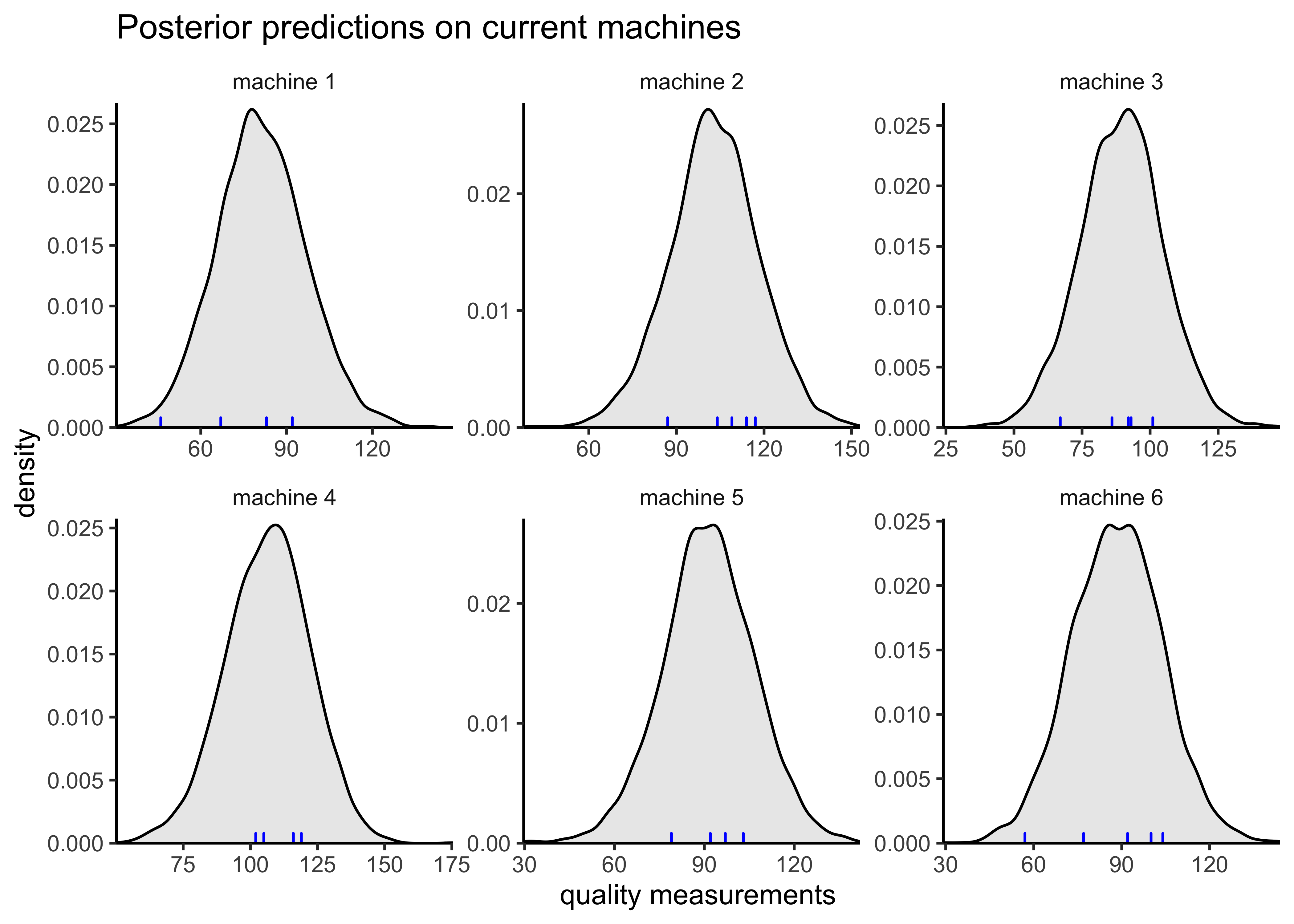
Calculate the expected utility for each current machine.
machine_utilities <- apply(factory_ypred, 2, utility)
tibble(
  machine = glue("machine {seq(length(machine_utilities))}"),
  expected_utility = machine_utilities
) %>%
kableExtra::kbl()| machine | expected_utility |
|---|---|
| machine 1 | -26.15 |
| machine 2 | 70.15 |
| machine 3 | 17.50 |
| machine 4 | 76.45 |
| machine 5 | 27.45 |
| machine 6 | 11.05 |
b) Rank the machines based on the expected utilities. In other words order the machines from worst to best. Also briefly explain what the utility values tell about the quality of these machines. E.g. Tell which machines are profitable and which are not (if any).
Based on their expected utility, the rankings of the machines from worst to best is: 1, 6, 3, 5, 2, 4. Machine 1 has a negative utility, indicating that it is expected to be unprofitable.
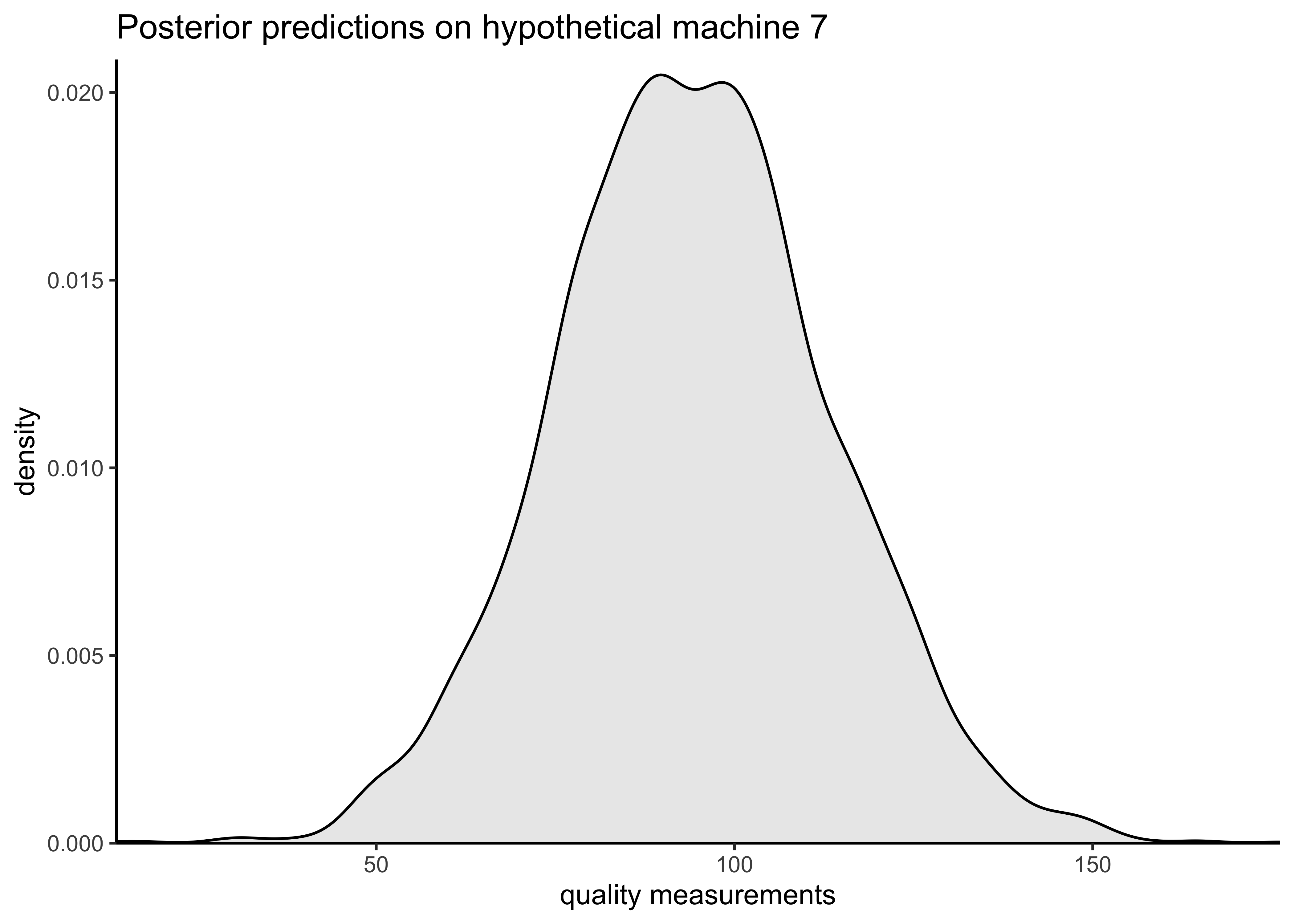
c) Compute and report the expected utility of the products of a new (7th) machine.
machine7_pred <- rstan::extract(hierarchical_model, pars = "y7pred")$y7pred

ggplot(tibble(x = unlist(machine7_pred)), aes(x = x)) +
  geom_density(fill = "black", alpha = 0.1) +
  scale_x_continuous(expand = expansion(c(0, 0))) +
  scale_y_continuous(expand = expansion(c(0, 0.02))) +
  labs(
    x = "quality measurements",
    y = "density",
    title = "Posterior predictions on hypothetical machine 7"
  )
# Expected utility from machine 7.
utility(machine7_pred)
#> [1] 30.7The expected utility of hypothetical machine 7 is 30.7.
d) Based on your analysis, discuss briefly whether the company owner should buy a new (7th) machine.
Based on this analysis, purchasing another machine would be expected to be profitable. It might be worth replacing machine 1 with this new machine.
e) As usual, remember to include the source code for both Stan and R (or Python).
The model is available here “assignment07_factories_hierarchical.stan”.
The only changes were made in the generated quantities block:
\\...
generated quantities {
  // Compute the predictive distribution for the sixth machine.
  real y6pred;  // Leave for compatibility with earlier assignments.
  vector[J] ypred;
  real mu7pred;
  real y7pred;
  vector[J] log_lik[N];

  y6pred = normal_rng(mu[6], sigma);
  for (j in 1:J) {
    ypred[j] = normal_rng(mu[j], sigma);
  }

  mu7pred = normal_rng(alpha, tau);
  y7pred = normal_rng(mu7pred, sigma);

  for (j in 1:J) {
    for (n in 1:N) {
      log_lik[n,j] = normal_lpdf(y[n,j] | mu[j], sigma);
    }
  }
}sessionInfo()#> R version 4.1.2 (2021-11-01)
#> Platform: x86_64-apple-darwin17.0 (64-bit)
#> Running under: macOS Big Sur 10.16
#>
#> Matrix products: default
#> BLAS: /Library/Frameworks/R.framework/Versions/4.1/Resources/lib/libRblas.0.dylib
#> LAPACK: /Library/Frameworks/R.framework/Versions/4.1/Resources/lib/libRlapack.dylib
#>
#> locale:
#> [1] en_US.UTF-8/en_US.UTF-8/en_US.UTF-8/C/en_US.UTF-8/en_US.UTF-8
#>
#> attached base packages:
#> [1] stats graphics grDevices datasets utils methods base
#>
#> other attached packages:
#> [1] forcats_0.5.1 stringr_1.4.0 dplyr_1.0.7
#> [4] purrr_0.3.4 readr_2.0.1 tidyr_1.1.3
#> [7] tibble_3.1.3 tidyverse_1.3.1 tidybayes_3.0.1
#> [10] rstan_2.21.2 ggplot2_3.3.5 StanHeaders_2.21.0-7
#> [13] glue_1.4.2
#>
#> loaded via a namespace (and not attached):
#> [1] matrixStats_0.61.0 fs_1.5.0 lubridate_1.7.10
#> [4] webshot_0.5.2 httr_1.4.2 rprojroot_2.0.2
#> [7] tensorA_0.36.2 tools_4.1.2 backports_1.2.1
#> [10] bslib_0.2.5.1 utf8_1.2.2 R6_2.5.0
#> [13] DBI_1.1.1 colorspace_2.0-2 ggdist_3.0.0
#> [16] withr_2.4.2 tidyselect_1.1.1 gridExtra_2.3
#> [19] prettyunits_1.1.1 processx_3.5.2 curl_4.3.2
#> [22] compiler_4.1.2 cli_3.0.1 rvest_1.0.1
#> [25] arrayhelpers_1.1-0 xml2_1.3.2 labeling_0.4.2
#> [28] bookdown_0.24 posterior_1.1.0 sass_0.4.0
#> [31] scales_1.1.1 checkmate_2.0.0 aaltobda_0.3.1
#> [34] callr_3.7.0 systemfonts_1.0.3 digest_0.6.27
#> [37] svglite_2.0.0 rmarkdown_2.10 pkgconfig_2.0.3
#> [40] htmltools_0.5.1.1 highr_0.9 dbplyr_2.1.1
#> [43] rlang_0.4.11 readxl_1.3.1 rstudioapi_0.13
#> [46] jquerylib_0.1.4 farver_2.1.0 generics_0.1.0
#> [49] svUnit_1.0.6 jsonlite_1.7.2 distributional_0.2.2
#> [52] inline_0.3.19 magrittr_2.0.1 kableExtra_1.3.4
#> [55] loo_2.4.1 Rcpp_1.0.7 munsell_0.5.0
#> [58] fansi_0.5.0 abind_1.4-5 lifecycle_1.0.0
#> [61] stringi_1.7.3 yaml_2.2.1 pkgbuild_1.2.0
#> [64] grid_4.1.2 parallel_4.1.2 crayon_1.4.1
#> [67] lattice_0.20-45 haven_2.4.3 hms_1.1.0
#> [70] knitr_1.33 ps_1.6.0 pillar_1.6.2
#> [73] codetools_0.2-18 clisymbols_1.2.0 stats4_4.1.2
#> [76] reprex_2.0.1 evaluate_0.14 V8_3.4.2
#> [79] renv_0.14.0 RcppParallel_5.1.4 modelr_0.1.8
#> [82] vctrs_0.3.8 tzdb_0.1.2 cellranger_1.1.0
#> [85] gtable_0.3.0 assertthat_0.2.1 xfun_0.25
#> [88] broom_0.7.9 coda_0.19-4 viridisLite_0.4.0
#> [91] ellipsis_0.3.2 here_1.0.1