19 Section 21. Notes on ‘Ch 23. Dirichlet process models’
2022-01-20
knitr::opts_chunk$set(echo = TRUE, dpi = 300, comment = "#>")

library(tidyverse)

theme_set(
  theme_bw() +
    theme(
      strip.background = element_blank(),
      axis.ticks = element_blank()
    )
)
These are just notes on a single chapter of BDA3 that were not part of the course.
19.1 Chapter 23. Dirichlet process models
- Dirichlet process: an infinite-dimensional generalization of the Dirichlet distribution
- used as a prior on unknown distributions
- can extend finite component mixture models to infinite mixture models
23.1 Bayesian histograms
- the histogram as a simple form of density estimation
- demonstrate a flexible parametric version that motivates the non-parametric in the following section
- prespecified knots: \(\xi = (\xi_0, \dots, \xi_k)\) with \(\xi_{n-1} < \xi_n\)
- probability model for the density (a histogram):
- where \(\pi = (\pi_1, \dots, \pi_k)\) is an unknown probability vector
\[ f(y) = \sum_{h=1}^k 1_{\xi_{h-1} < y \le \xi_h} \frac{\pi_h}{(\xi_h - \xi_{h-1})} \]
- prior for the probabilities \(\pi\) as a Dirichlet distribution:
\[ p(\pi|a) = \frac{\Gamma(\sum_{h=1}^k a_h)}{\prod_{h=1}^k \Gamma(a_h)} \prod_{h=1}^k \pi _h^{a_h - 1} \]
- replace the hyperparameter vector: \(a = \alpha \pi_0\) where \(\pi_0\) is:
\[ \text{E}(\pi|a) = \pi_0 = \left( \frac{a_1}{\sum_h a_h}, \dots, \frac{a_k}{\sum_h a_h} \right) \]
- the posterior for \(\pi\) becomes:
- where \(n_i\) is the number of observations \(y\) in the \(i\)th bin
\[ p(\pi | y) \propto \prod_{h=1}^k \pi_h^{a_h + n_h - 1} = \text{Dirichlet}(a_1 + n_1, \dots, a_k + n_k) \]
- this histogram estimator does well but is sensitive to the specification of the knots
23.2 Dirichlet process prior distributions
Definition and basic properties
- goal is to not need to prespecify the bins of the histogram
- let:
- \(\Omega\): sample space
- \(B_1, \dots, B_k\): measure subsets of \(\Omega\)
- if \(\Omega = \Re\), then \(B_1, \dots, B_k\) are non-overlapping intervals that partition the real line into a finite number of bins
- \(P\): unknown probability measure of \((\Omega, \mathcal{B})\)
- \(\mathcal{B}\): “collection of all possible subsets of the sample space \(\Omega\)”
- \(P\) assigns probabilities to the subsets \(\mathcal{B}\)
- probability for a set of bins \(B_1, \dots, B_k\) partitioning \(\Omega\):
\[ P(B_1), \dots, P(B_k) = \left( \int_{B_1} f(y) dy, \dots, \int_{B_k} f(y) dy \right) \]
- \(P\) is a random probability measure (RPM), so the bin probabilities are random variables
- a good prior for the bin probabilities is the Dirichlet distribution @ref(eq:dirichlet-prior
- where \(P_0\) is a base probability measure providing the initial guess at \(P\)
- where \(\alpha\) is a prior concentration parameter
- controls shrinkage of \(P\) towards \(P_0\)
\[ P(B_1), \dots, P(B_k) \sim \text{Dirichlet}(\alpha P_0(B_1), \dots, \alpha P_0(B_k)) \tag{19.1} \]
- difference with previous Bayesian histogram: only specifies that bin \(B_k\) is assigned probability \(P(B_k)\) and not how probability mass is distributed across the bin \(B_k\)
- thus, for a fixed set s of bins, this equation does not full specify the prior for \(P\)
- need to eliminate the sensitivity to the choice of bins by assuming the prior holds for all possible partitions \(B_1, \dots, B_k\) for all \(k\)
- then it is a fully specified prior for \(P\)
- “must exist a random probability measure \(P\) such that the probabilities assigned to any measurable partition \(B_1, \dots, B_k\) by \(P\) is \(\text{Dirichlet}(\alpha P_0(B_1), \dots, \alpha P_0(B_k))\)”
- the resulting \(P\) is a Dirichlet process:
- \(P \sim \text{DP}(\alpha P_0)\)
- \(\alpha > 0\): a scalar precision parameter
- \(P_0\): baseline probability measure also on \((\Omega, \mathcal{B})\)
- the resulting \(P\) is a Dirichlet process:
- implications of DP:
- the marginal random probability assigned to any subset \(B\) is a beta distribution
- \(P(B) \sim \text{Beta}(\alpha PP_0(B), \alpha (1-P_0(B)))\) for all \(B \in \mathcal{B}\)
- the prior for \(P\) is centered on \(P_0\): \(E(P(B)) = P_0(B)\)
- \(\alpha\) controls variance
- \(\text{var}(P(B)) = \frac{P_0(B)(1 - P_0(B))}{1 + \alpha}\)
- the marginal random probability assigned to any subset \(B\) is a beta distribution
- get posterior for \(P\):
- let \(y_i \stackrel{iid}{\sim} P\) fir \(i = 1, \dots, n\)
- \(P \sim \text{DP}(\alpha P_0)\)
- \(P\) denotes the probability measure and its corresponding distribution
- from (19.1), for any partition \(B_1, \dots, B_k\):
\[ p(B_1), \dots, P(B_k) | y_1, \dots, y_k \sim \text{Dirichlet} \left( \alpha P_0(B_1) + \sum_{i=1}^n 1_{y_i \in B_1}, \dots, \alpha P_0(B_k) + \sum_{i=1}^n 1_{y_i \in B_k} \right) \]
- this can be converted to the following:
\[ P | y_1, \dots, y_n \sim \text{DP} \left( \alpha P_0 \sum_i \delta_{y+i} \right) \]
- finally, the posterior expectation of \(P\):
\[ \text{E}(P(B) | y^n) = \left(\frac{\alpha}{\alpha + n} \right) P_0(B) + \left(\frac{n}{\alpha + n} \right) \sum_{i=1}^n \frac{1}{n} \delta_{y_i} \tag{19.2} \]
- DP is a model similar to a random histogram but without dependence on the bins
- cons of a DP prior:
- lack of smoothness
- induces negative correlation between \(P(B_1)\) and \(P(B_2)\) for any two disjoint bins with no account for the distance between them
- realizations from the DP are discrete distributions
- with \(P \sim \text{DP}(\alpha P_0)\), \(P\) is atomic and have nonzero weights only on a set of atoms, not a continuous density on the real line
Stick-breaking construction
- more intuitive understanding of DP
- induce \(P \sim \text{DP}(\alpha P_0)\) by letting:
\[ \begin{aligned} P(\cdot) &= \sum_{h=1}^{\infty} \pi_h \delta_{\theta_h}(\cdot) \\ \pi_h &= V_h \prod_{l<h} (1 - V_i) \\ V_h &\sim \text{Beta}(1, \alpha) \\ \theta_h &\sim P_0 \end{aligned} \]
- where:
- \(P_0\): base distribution
- \(\delta_\theta\): degenerate distribution with all mass at \(\theta\)
- \((\theta_h)_{h=1}^{\infty}\): the atoms generated independently by from \(P_0\)
- the atoms are generated by the stick-breaking process
- this ensures the weights sum to 1
- \(\pi_h\): probability mass at atom \(\theta_h\)
- the stick-breaking process:
- start with a stick of length 1
- represents the total probability allocated to all the atoms
- break off a random piece of length \(V_1\) determined by a draw from \(\text{Beta}(1, \alpha)\)
- set \(\pi_1 = V_1\) as the probability weight to the randomly generated first atom \(\theta_1 \sim P_0\)
- break off another piece of the remaining stick (now length \(1-V_1\)): \(V_2 \sim \text{Beta}(1, \alpha)\)
- set \(\pi_2 = V_2(1-V_1)\) as the probability weight to the next atom \(\theta_2 \sim P_0\)
- repeat until the stick is fully used
- start with a stick of length 1
- implications:
- during the process, the stick get shorter, so lengths allocated to later indexed atoms decrease stochastically
- rate of decrease of stick length depends on \(\alpha\)
- \(\alpha\) near 0 lead to high weights early on
- below are realizations of the stick breaking process
- set \(P_0\) as a standard normal distribution and vary \(\alpha\)
stick_breaking_process <- function(alpha, n = 1000) {
  theta <- rnorm(n, 0, 1) # P0 = standard normal
  vs <- rbeta(n, 1, alpha)
  pi <- rep(0, n)
  pi[1] <- vs[1]
  stick <- 1.0 - vs[1]
  for (h in 2:n) {
    pi[h] <- vs[h] * stick
    stick <- stick - pi[h]
  }
  return(list(theta = theta, pi = pi))
}

dp_realization <- stick_breaking_process(10)
sum(dp_realization$pi)
#> [1] 1set.seed(549)
tibble(alpha = c(0.5, 1, 5, 10)) %>%
mutate(
dp = purrr::map(alpha, stick_breaking_process, n = 1000),
theta = purrr::map(dp, ~ .x$theta),
pi = purrr::map(dp, ~ .x$pi)
) %>%
select(-dp) %>%
unnest(c(theta, pi)) %>%
ggplot(aes(x = theta, y = pi)) +
facet_wrap(vars(alpha), nrow = 2, scales = "fixed") +
geom_col(width = 0.05) +
scale_x_continuous(expand = expansion(c(0.02, 0.02))) +
scale_y_continuous(expand = expansion(c(0, 0.02))) +
labs(x = "\u03B8", y = "\u03C0")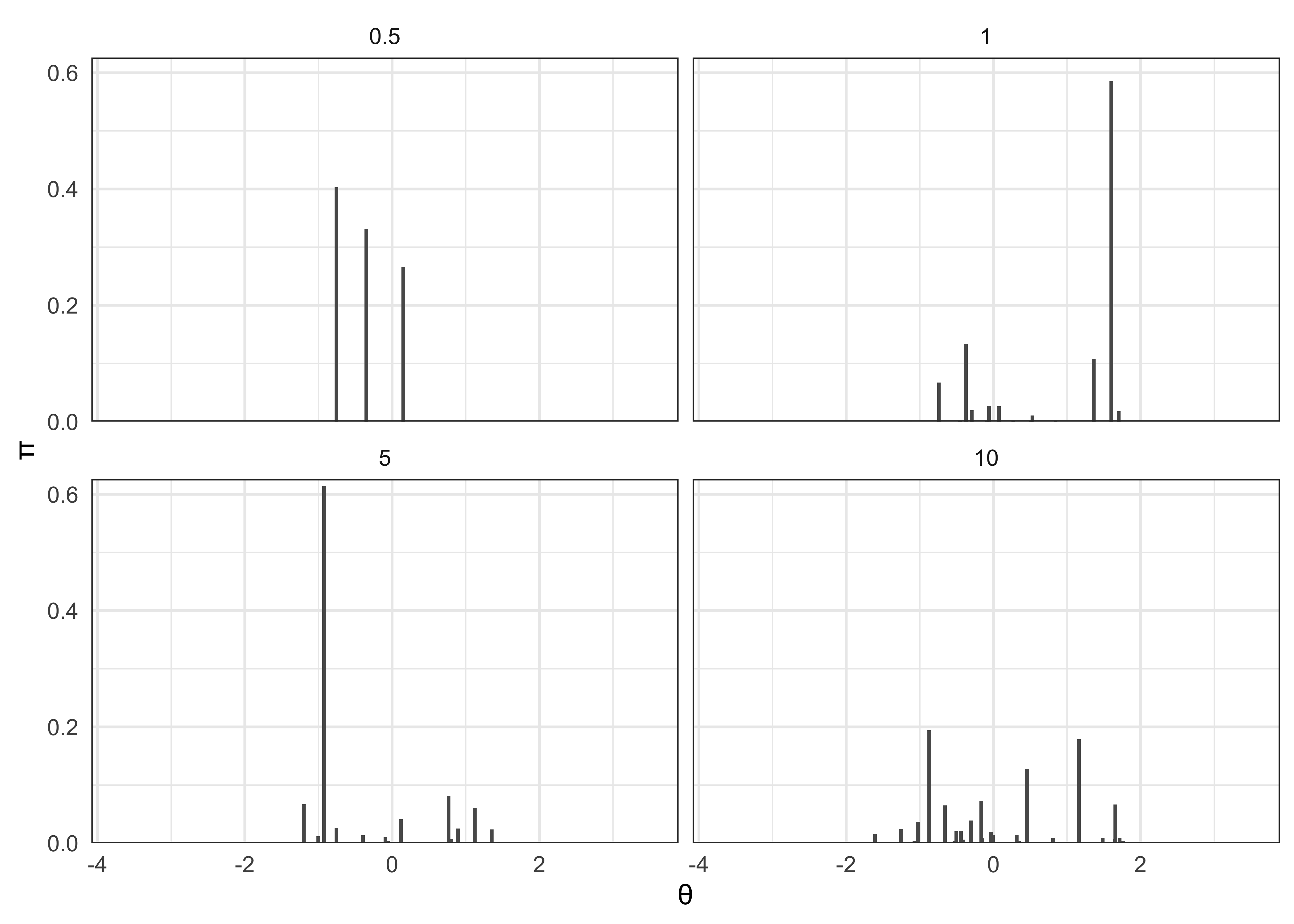
23.3 Dirichlet process mixtures
Specification and Polya urns
- “the DP is more appropriately used as a prior for an unknown mixture of distributions” (pg 549)
- in the case of density estimation, a general kernel mixture model can be specified as (19.3)
- \(\mathcal{K}(\cdot | \theta)\): a kernel
- \(\theta\): location and possibly scale parameters
- \(P\): “mixing measure”
\[ f(y|P) = \int \mathcal{K}(y|\theta) d P(\theta) \tag{19.3} \]
- treating \(P\) as discrete results in a finite mixture model
- setting a prior on \(P\) creates an infinite mixture model
- prior: \(P \sim \pi_\mathcal{P}\)
- \(\mathcal{P}\): space of all probability measures on \((\Omega, \mathcal{B})\)
- \(\pi_\mathcal{P}\): the prior over the space defined by \(\mathcal{P}\)
- prior: \(P \sim \pi_\mathcal{P}\)
- if set \(\pi_\mathcal{P}\) as a DP prior, results in a DP mixture model
\[ f(y) = \sum_{h=1}^\infty \pi_h \mathcal{K}(y | \theta_h^*) \tag{19.4} \]
- equation (19.4) resembles a finite mixture model except the number of mixture components in set to infinity
- does not mean there will be infinite number of components
- instead the model is just flexible to add more mixture components if necessary
- consider the following specification
- issue of how to conduct posterior computation with a DP mixture (DPM) because \(P\) has infinitely many parameters
\[ y_i \sim \mathcal{K}(\theta_i) \text{,} \quad \theta_i \sim P \text{,} \quad P \sim \text{DP}(\alpha P_0) \]
- can marginalize out \(P\) to get an induced prior on the subject-specific parameters \(\theta^n = (\theta_1, \dots, \theta_n)\)
- results in the Polya urn predictive rule:
\[ p(\theta_i | \theta_1, \dots, \theta_{i-1}) \sim \left( \frac{\alpha}{\alpha + i -1} \right) P_0(\theta_i) + \sum_{j=1}^{i-1} \left( \frac{1}{\alpha + i - 1} \right) \delta_{\theta_j} \tag{19.5} \]
- Chinese restaurant process as a metaphor for the Polya urn predictive rule (19.5):
- consider a restaurant with infinitely many tables
- the first customers sits at a table with dish \(\theta_1^*\)
- the second customer sits at the first table with probability \(\frac{1}{1+\alpha}\) or a new table with probability \(\frac{\alpha}{1+\alpha}\)
- repeat this process for the \(i\)th customer:
- sit at an occupied table with probability \(\frac{c_j}{1 - i + \alpha}\) where \(c_j\) is the number of customers already at the table -sit at a new table with probability \(\frac{\alpha}{n-i+\alpha}\)
- interpretation:
- each table represents a cluster of subjects
- the number of clusters depends on the number of subjects
- makes sense to have the possibility of more clusters with more subjects (instead of a fixed number of clusters as in a finite mixture model)
- there is a description of the sampling process for the posterior of \(\theta_i | \theta_{-i}\)
Hyperprior distribution
- \(\alpha\): the DP precision parameter
- plays a role in controlling the prior on the number of clusters
- small, fixed \(\alpha\) favors allocation to few clusters (relative to sample size)
- if \(\alpha=1\), the prior indicates that two randomly selected subjects have a 50/50 chance of belonging to the same cluster
- alternatively can set a hyperprior on \(\alpha\) and let the data inform the value
- common to use a Gamma distribution: \(\Gamma(a_\alpha, b_\alpha)\)
- authors indicate that setting a hyperprior on \(\alpha\) tends to work well in practice
- \(P_0\): base probability for the DP
- can think of \(P_0\) as setting the prior for the cluster locations
- can put hyperpriors on \(P_0\) parameters
23.4 Beyond density estimation
Nonparametric residual distributions
- “The real attraction of Dirichlet process mixture (DPM) models is that they can be used much more broadly for relaxing parametric assumptions in hierarchical models.” (pg 557)
- consider the linear regression with a nonparametric error distribution (19.6)
- \(X_i = (X_{i1}, \dots, X_{ip})\): vector of predictors
- \(\epsilon_i\): error term with distribution \(f\)
\[ y_i = X_i \beta + \epsilon_i \text{,} \quad \epsilon_i \sim f \tag{19.6} \]
- can relax the assumption that \(f\) has parametric form
\[ \epsilon_i \sim N(0, \phi_i^{-1}) \text{,} \quad \phi \sim P \text{,} \quad P \sim \text{DP}(\alpha P_0) \]
Nonparametric models for parameters that vary by group
- consider hierarchical linear models with varying coefficients
- can account for uncertainty about the distribution of coefficients by placing a DP or DPM priors on them
- where:
- \(y_i = (y_{i1}, \dots, y_{in_i})\): repeated measurements for item \(i\)
- \(\mu_i\): subject-specific mean
- \(\epsilon_{ij}\): observation specific residual
\[ y_{ij} = \mu_i + \epsilon_{ij} \text{,} \quad \mu_i \sim f \text{,} \quad \epsilon_{ij} \sim g \tag{19.7} \]
- typically for (19.7):
- \(f \equiv N(\mu, \phi^{-1})\)
- \(g \equiv N(0, \sigma^2)\)
- can let more flexibility in characterizing variability among subjects:
- \(\mu_i \sim P \text{,} \quad P \sim \text{DP}(\alpha P_0)\)
- the DP prior induces a latent class model
- the subjects are grouped into an unknown number of clusters (19.8)
- \(S_i \in \{1, \dots, \infty\}\): latent class index
- \(\pi_h\): probability of allocation to latent class \(h\)
\[ \mu_i = \mu^*_{S_i} \text{,} \quad \Pr(S_i = h) = \pi_h \text{,} \quad h = 1, 2, \dots \tag{19.8} \]
There is more to this chapter, but it is currently beyond my understanding. I hope to return to this chapter later with a better understanding of Dirichlet processes in the future.
sessionInfo()#> R version 4.1.2 (2021-11-01)
#> Platform: x86_64-apple-darwin17.0 (64-bit)
#> Running under: macOS Big Sur 10.16
#>
#> Matrix products: default
#> BLAS: /Library/Frameworks/R.framework/Versions/4.1/Resources/lib/libRblas.0.dylib
#> LAPACK: /Library/Frameworks/R.framework/Versions/4.1/Resources/lib/libRlapack.dylib
#>
#> locale:
#> [1] en_US.UTF-8/en_US.UTF-8/en_US.UTF-8/C/en_US.UTF-8/en_US.UTF-8
#>
#> attached base packages:
#> [1] stats graphics grDevices datasets utils methods base
#>
#> other attached packages:
#> [1] forcats_0.5.1 stringr_1.4.0 dplyr_1.0.7 purrr_0.3.4
#> [5] readr_2.0.1 tidyr_1.1.3 tibble_3.1.3 ggplot2_3.3.5
#> [9] tidyverse_1.3.1
#>
#> loaded via a namespace (and not attached):
#> [1] Rcpp_1.0.7 lubridate_1.7.10 clisymbols_1.2.0 assertthat_0.2.1
#> [5] digest_0.6.27 utf8_1.2.2 R6_2.5.0 cellranger_1.1.0
#> [9] backports_1.2.1 reprex_2.0.1 evaluate_0.14 httr_1.4.2
#> [13] highr_0.9 pillar_1.6.2 rlang_0.4.11 readxl_1.3.1
#> [17] rstudioapi_0.13 jquerylib_0.1.4 rmarkdown_2.10 labeling_0.4.2
#> [21] munsell_0.5.0 broom_0.7.9 compiler_4.1.2 modelr_0.1.8
#> [25] xfun_0.25 pkgconfig_2.0.3 htmltools_0.5.1.1 tidyselect_1.1.1
#> [29] bookdown_0.24 fansi_0.5.0 crayon_1.4.1 tzdb_0.1.2
#> [33] dbplyr_2.1.1 withr_2.4.2 grid_4.1.2 jsonlite_1.7.2
#> [37] gtable_0.3.0 lifecycle_1.0.0 DBI_1.1.1 magrittr_2.0.1
#> [41] scales_1.1.1 cli_3.0.1 stringi_1.7.3 farver_2.1.0
#> [45] renv_0.14.0 fs_1.5.0 xml2_1.3.2 bslib_0.2.5.1
#> [49] ellipsis_0.3.2 generics_0.1.0 vctrs_0.3.8 tools_4.1.2
#> [53] glue_1.4.2 hms_1.1.0 yaml_2.2.1 colorspace_2.0-2
#> [57] rvest_1.0.1 knitr_1.33 haven_2.4.3 sass_0.4.0