7 Section 7. Hierarchical models and exchangeability

Exchangeability vs. independence

• exchangeability and independence are two separate concepts; neither necessarily implies the other
  • independent identically distributed variables/parameters are exchangeable
  • exchangeability is less strict condition than independence

Weakly informative priors for hierarchical variance parameters

• suggestions have changed since writing section 5.7
  • section 5.7 recommends use of half-Cauchy as weakly informative prior for hierarchical variance parameters
  • now recommend a “half-normal if you have substantial information on the high end values, or or half-\(t_4\) if you there might be possibility of surprise”
  • “half-normal produces usually more sensible prior predictive distributions and is thus better justified”
  • “half-normal leads also usually to easier inference”

1. Constructing a parameterized prior distribution

• have historical data to inform our model
  • can use it to construct a prior for our new data or use it as data to inform the posterior
  • probably should not use it for both though, thus favor using it directly in the model alongside our new data
• for each experiment \(j\), with data \(y_j\), estimate the parameter \(\theta_j\)
  • the parameters \(\theta_j\) can come from a population distribution parameterized by \(\text{Beta}(\alpha, \beta)\)

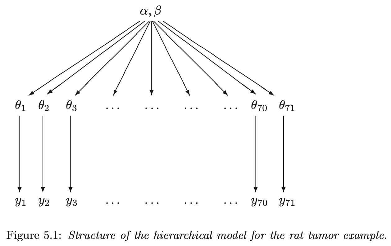
hierarchical structure graph

5.2 Exchangeability and hierarchical models

• if no information (other than \(y\)) is available to distinguish any of the \(\theta_j\)’s, and no ordering (time) or grouping can be made, then we must assume symmetry among the parameters in the prior distribution
  • this symmetry is represented probabilistically by exchangeability: the parameters \((\theta_1, \dots, \theta_J)\) are exchangeable in the join distribution if \(p(\theta_1, \dots, \theta_J)\) is invariant to permutations of the indices \((1, \dots, J)\)
• “in practice, ignorance implies exchangeability” (pg. 104)
  • the less we know about a problem, the more confident we can claim exchangeability (i.e. we don’t know any better)
• exchangeability is not the same as i.i.d:
  • probability of a die landing on each face: parameters \((\theta_1, \dots, \theta_6)\) are exchangeable because we think the faces are all the same, but they are not independent because the total must sum to 1
• exchangeability when additional information is available on the groups
  • if the observations can be grouped in their own submodels, but the group properties are unknown, can make a common prior distribution for the group properties
  • if \(y_i\) has additional information \(x_i\) so that \(y_i\) are not exchangeable, but \((y_i, x_i)\) are exchangeable, we can make a join model for \((y_i, x_i)\) or a conditional model \(y_i | x_i\)
• the usual way to model exchangeability with covariates is through conditional independence

\[ p(\theta_1, \dots, \theta_J | x_1, \dots, x_J) = \int [\prod_{j=1}^J p(\theta_j | \phi, x_j)] p(\phi|x) d \phi \]

• \(phi\) is unknown, so it gets a prior distribution, too \(p(\phi)\)
  • the posterior distribution is of the vector \((\phi, \theta)\)
  • thus the joint prior is: \(p(\phi, \theta) = p(\phi) p(\theta|\phi)\)
• joint posterior:

\[ \begin{aligned} p(\phi, \theta | y) &\propto p(\phi, \theta) p(y|\phi, \theta) \\ &= p(\phi, \theta) p(y|\theta) \end{aligned} \]

• posterior predictive distributions
  • get predictions on both levels

5.3 Bayesian analysis of conjugate hierarchical models

• analysis derivation of conditional and marginal distributions
  1. write the (unnormalized) joint posterior density \(p(\theta, \phi | y)\) as a product of the hyperprior \(p(\phi)\), the population distribution \(p(\theta|\phi)\) and the likelihood \(p(y|\theta)\)
  2. determine the conditional posterior density of \(\theta\) given \(\phi\): \(p(\theta | \phi, y)\)
  3. estimate \(\phi\) from its marginal posterior distribution \(p(\phi|y)\)
• drawing simulations from the posterior distribution
  1. draw \(\phi\) from \(p(\phi|y)\)
  2. draw \(\theta\) from its conditional posterior distribution \(p(\theta | \phi, y)\) using the values of \(\phi\) from the previous step
  3. draw predictive values \(\tilde{y}\) given the values of \(\theta\)
• example on rat tumors is a good demonstration of the shrinkage of parameter estimates in a hierarchical model
  • the 1:1 line represents where the posteriors would be for a non-pooling model
  • can see the shrinkage of the extreme values towards the average
  • the effect is stronger for experiments with fewer rats

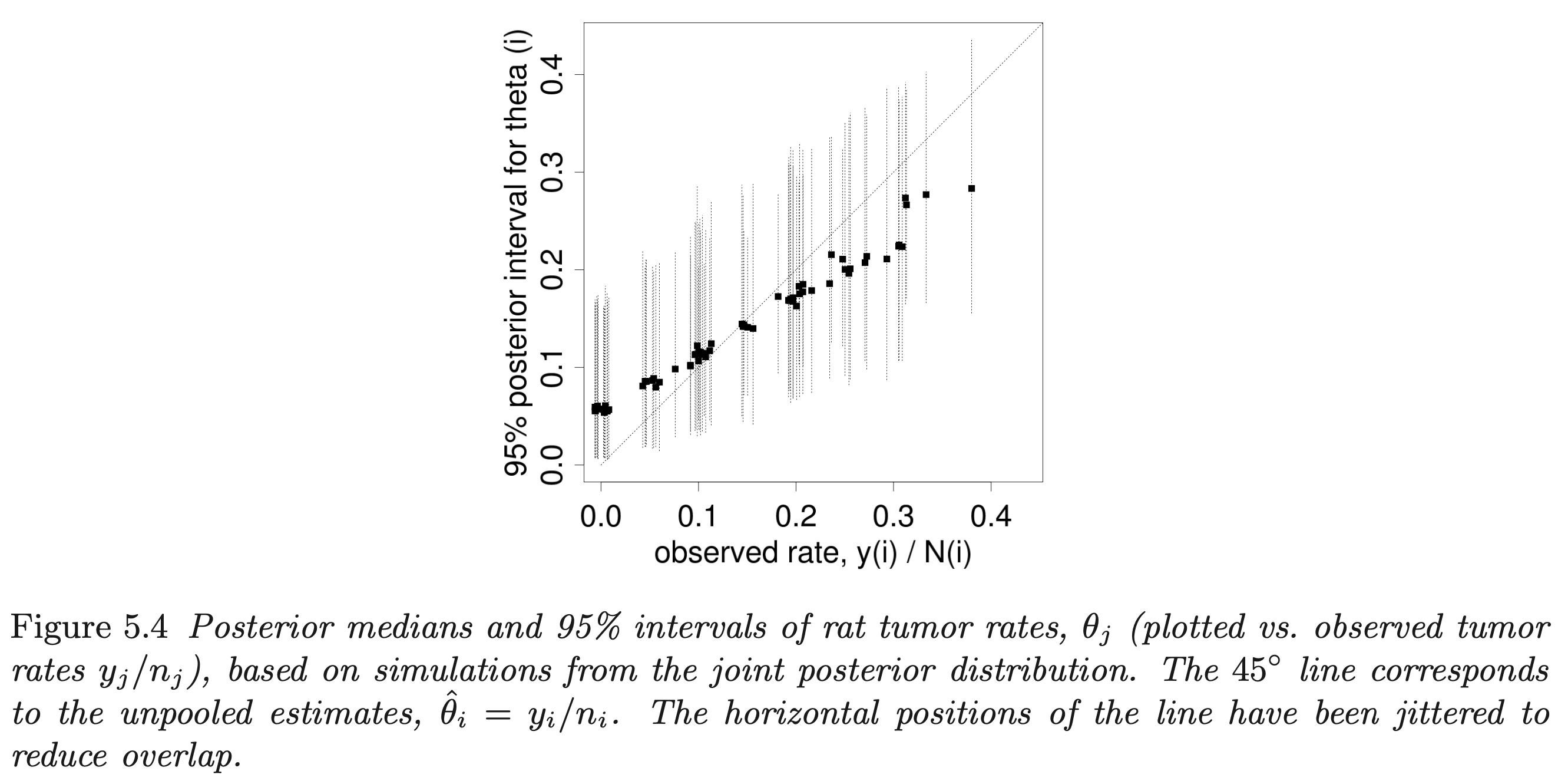
rat tumor model posterior

5.4 Normal model with exchangeable parameters

• drawing posterior predictive samples:
  1. for new data \(\tilde{y}\) of existing groups \(J\), use the posterior distributions for \((\theta_1, \dots, \theta_j)\)
  2. for new data \(\tilde{y}\) for \(\tilde{J}\) new groups:
  3. draw values for the hyperparameters \(\mu, \tau\) (in this case)
  4. draw \(\tilde{J}\) new parameters \((\tilde{\theta}_1, \dots, \tilde{\theta}_\tilde{J})\) from \(p(\tilde{\theta} | \mu, \tau)\)
  5. draw \(\tilde{y}\) given \(\tilde{\theta}\)

5.5 Example: parallel experiments in eight schools

• a full example of a Bayesian hierarchical modeling process and analysis

5.6 Hierarchical modeling applied to a meta-analysis

• another good example of analyzing the results of a Bayesian hierarchical model
  • notes the importance of interpreting both the mean and standard error hyperparameters to interpret the distribution of possible parameter values

5.7 Weakly informative priors for variance parameters

• “It turns out the the choice of ‘noninformative’ prior distribution can have a big effect on inferences,” (pg. 128)
  • uniform prior distributions will often lead to overly-dispersed posteriors
    • this is especially true for the standard error term of a hyperparameter when there are few groups
  • half-Cauchy is often a good balance between restricting the prior to reasonable value but with fat enough tails to allow for uncertainty
    • particularly good for variance parameters of hierarchical models with few groups

‘7.1. Hierarchical models’

• description of the diagram of a hierarchical model
  • box: known value
    • double box: indicates a fixed experimental value (e.g. decided how many rats to include in an experiment)
  • circle: unknown parameter
  • box with the subscript \(j\): indicates that everything within the box is repeated \(J\) times

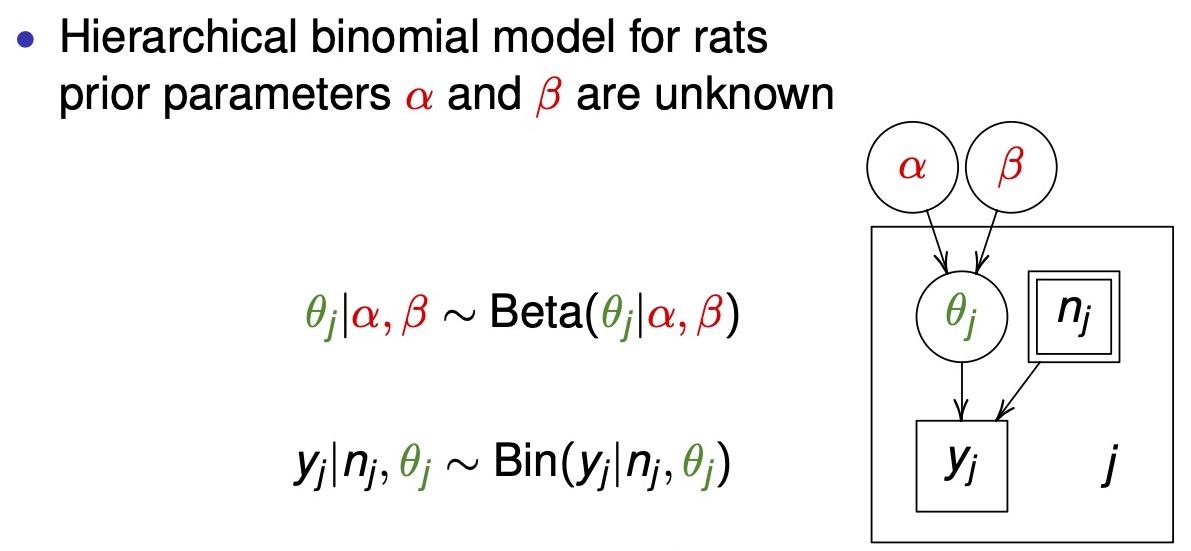
hierarchical box diagram

• hierarchical model shrinkage effects with sample size
  • below example shows how shrinkage is stronger for data points with smaller sample size (county radon example)

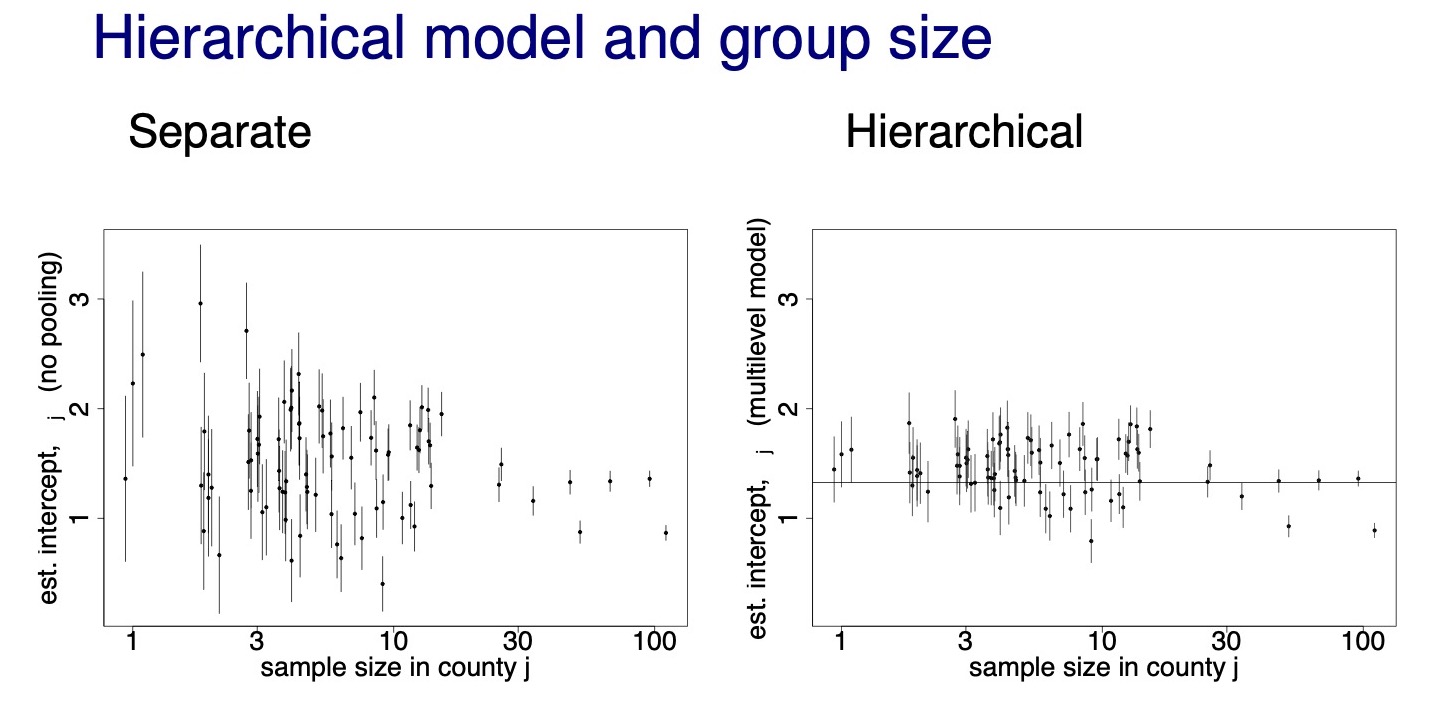
chrinkage with sample size

• below, I replicate the 8-schools model in Stan and try to make the plot of \(\theta\) over \(\tau\)

schools_data <- list(
  J = 8,
  y = c(28, 8, -3, 7, -1, 1, 18, 12),
  sigma = c(15, 10, 16, 11, 9, 11, 10, 18)
)

eight_schools <- stan(
  file = here::here("models", "8-schools.stan"),
  data = schools_data,
  chains = 4,
  warmup = 1000,
  iter = 2000,
  cores = 2,
  refresh = 0
)

eight_schools

#> Inference for Stan model: 8-schools.
#> 4 chains, each with iter=2000; warmup=1000; thin=1; 
#> post-warmup draws per chain=1000, total post-warmup draws=4000.
#> 
#>            mean se_mean   sd   2.5%    25%    50%    75%  97.5% n_eff Rhat
#> mu         7.93    0.10 5.11  -2.36   4.67   7.87  11.05  18.19  2776    1
#> tau        6.51    0.13 5.48   0.18   2.45   5.28   9.10  20.66  1651    1
#> eta[1]     0.37    0.01 0.97  -1.62  -0.26   0.38   1.04   2.22  4447    1
#> eta[2]     0.01    0.01 0.86  -1.71  -0.54   0.00   0.56   1.73  5131    1
#> eta[3]    -0.20    0.01 0.91  -2.00  -0.80  -0.22   0.41   1.61  5300    1
#> eta[4]    -0.04    0.01 0.88  -1.80  -0.63  -0.05   0.55   1.70  4508    1
#> eta[5]    -0.33    0.01 0.86  -1.98  -0.91  -0.36   0.23   1.43  4005    1
#> eta[6]    -0.20    0.01 0.89  -1.95  -0.79  -0.21   0.37   1.63  4784    1
#> eta[7]     0.33    0.01 0.90  -1.49  -0.27   0.38   0.93   2.07  4682    1
#> eta[8]     0.05    0.01 0.92  -1.78  -0.54   0.06   0.66   1.87  5721    1
#>  [ reached getOption("max.print") -- omitted 9 rows ]
#> 
#> Samples were drawn using NUTS(diag_e) at Wed Feb  9 06:38:55 2022.
#> For each parameter, n_eff is a crude measure of effective sample size,
#> and Rhat is the potential scale reduction factor on split chains (at 
#> convergence, Rhat=1).

theta_tau_post <- eight_schools %>%
  spread_draws(theta[school], tau) %>%
  mutate(school = purrr::map_chr(school, ~ LETTERS[[.x]]))

theta_tau_post %>%
  filter(tau < 20) %>%
  arrange(tau) %>%
  ggplot(aes(x = tau, y = theta, color = school)) +
  geom_smooth(
    method = "loess", formula = "y ~ x", n = 250, size = 0.8, alpha = 0.1
  ) +
  scale_x_continuous(expand = expansion(c(0, 0))) +
  scale_y_continuous(expand = expansion(c(0.02, 0.02))) +
  scale_color_brewer(type = "qual", palette = "Set1") +
  theme_classic()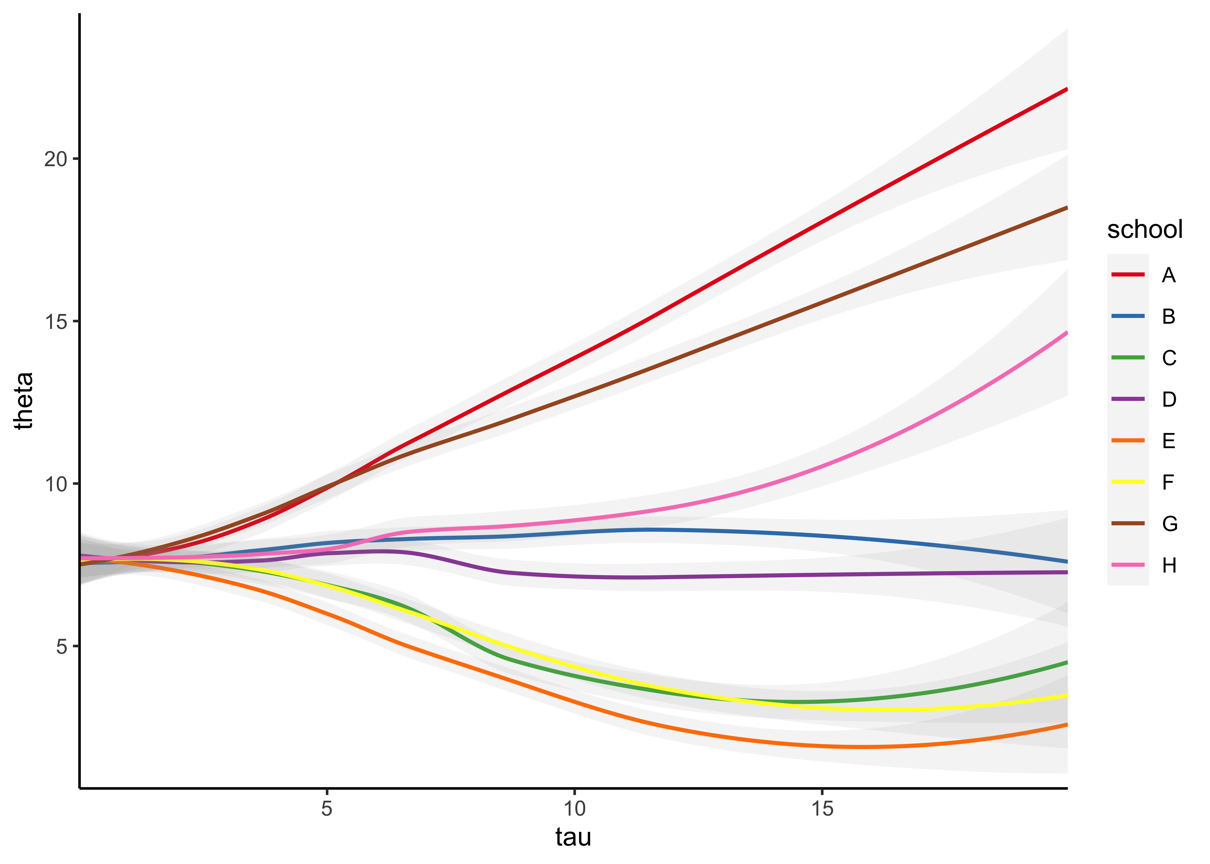

‘7.2. Exchangeability’

• exchangeability: parameters \(\theta_1, \dots ,\theta_J\) (or observations \(y_1, \dots , y_J\)) are exchangeable if the joint distribution \(p\) is invariant to the permutation of indices \((1, \dots, J)\)
  • e.g.: \(p(\theta_1, \theta_2, \theta_3) = p(\theta_2, \theta_3, \theta_1)\)
• exchangeability implies symmetry
  • if there is no information which can be used a priori to separate \(\theta_j\) form each other, we can assume exchangeability
  • ”Ignorance implies exchangeability”

sessionInfo()

#> R version 4.1.2 (2021-11-01)
#> Platform: x86_64-apple-darwin17.0 (64-bit)
#> Running under: macOS Big Sur 10.16
#> 
#> Matrix products: default
#> BLAS:   /Library/Frameworks/R.framework/Versions/4.1/Resources/lib/libRblas.0.dylib
#> LAPACK: /Library/Frameworks/R.framework/Versions/4.1/Resources/lib/libRlapack.dylib
#> 
#> locale:
#> [1] en_US.UTF-8/en_US.UTF-8/en_US.UTF-8/C/en_US.UTF-8/en_US.UTF-8
#> 
#> attached base packages:
#> [1] stats     graphics  grDevices datasets  utils     methods   base     
#> 
#> other attached packages:
#>  [1] forcats_0.5.1        stringr_1.4.0        dplyr_1.0.7         
#>  [4] purrr_0.3.4          readr_2.0.1          tidyr_1.1.3         
#>  [7] tibble_3.1.3         tidyverse_1.3.1      tidybayes_3.0.1     
#> [10] rstan_2.21.2         ggplot2_3.3.5        StanHeaders_2.21.0-7
#> 
#> loaded via a namespace (and not attached):
#>  [1] nlme_3.1-153         matrixStats_0.61.0   fs_1.5.0            
#>  [4] lubridate_1.7.10     RColorBrewer_1.1-2   httr_1.4.2          
#>  [7] rprojroot_2.0.2      tensorA_0.36.2       tools_4.1.2         
#> [10] backports_1.2.1      bslib_0.2.5.1        utf8_1.2.2          
#> [13] R6_2.5.0             mgcv_1.8-38          DBI_1.1.1           
#> [16] colorspace_2.0-2     ggdist_3.0.0         withr_2.4.2         
#> [19] tidyselect_1.1.1     gridExtra_2.3        prettyunits_1.1.1   
#> [22] processx_3.5.2       curl_4.3.2           compiler_4.1.2      
#> [25] cli_3.0.1            rvest_1.0.1          arrayhelpers_1.1-0  
#> [28] xml2_1.3.2           labeling_0.4.2       bookdown_0.24       
#> [31] posterior_1.1.0      sass_0.4.0           scales_1.1.1        
#> [34] checkmate_2.0.0      callr_3.7.0          digest_0.6.27       
#> [37] rmarkdown_2.10       pkgconfig_2.0.3      htmltools_0.5.1.1   
#> [40] highr_0.9            dbplyr_2.1.1         rlang_0.4.11        
#> [43] readxl_1.3.1         rstudioapi_0.13      jquerylib_0.1.4     
#> [46] farver_2.1.0         generics_0.1.0       svUnit_1.0.6        
#> [49] jsonlite_1.7.2       distributional_0.2.2 inline_0.3.19       
#> [52] magrittr_2.0.1       loo_2.4.1            Matrix_1.3-4        
#> [55] Rcpp_1.0.7           munsell_0.5.0        fansi_0.5.0         
#> [58] abind_1.4-5          lifecycle_1.0.0      stringi_1.7.3       
#> [61] yaml_2.2.1           pkgbuild_1.2.0       grid_4.1.2          
#> [64] parallel_4.1.2       crayon_1.4.1         lattice_0.20-45     
#> [67] splines_4.1.2        haven_2.4.3          hms_1.1.0           
#> [70] knitr_1.33           ps_1.6.0             pillar_1.6.2        
#> [73] codetools_0.2-18     clisymbols_1.2.0     stats4_4.1.2        
#> [76] reprex_2.0.1         glue_1.4.2           evaluate_0.14       
#> [79] V8_3.4.2             renv_0.14.0          RcppParallel_5.1.4  
#> [82] modelr_0.1.8         vctrs_0.3.8          tzdb_0.1.2          
#> [85] cellranger_1.1.0     gtable_0.3.0         assertthat_0.2.1    
#> [88] xfun_0.25            broom_0.7.9          coda_0.19-4         
#> [91] ellipsis_0.3.2       here_1.0.1