30 Chapter 2 Exercises
2021-08-19
30.1 Setup
knitr::opts_chunk$set(echo = TRUE, comment = "#>", dpi = 300)

rfiles <- list.files(here::here("src"), full.names = TRUE, pattern = "R$")
for (rfile in rfiles) {
  source(rfile)
}

library(glue)
library(tidyverse)
Complete questions 2.1-2.5, 2.8, 2.9, 2.14, 2.17, and 2.22.
30.2 Question 1
Posterior inference: suppose you have a \(\text{Beta}(4,4)\) prior distribution on the probability \(\theta\) that a count will yield a ‘head’ when spun. The coin is spun 10 times and ‘heads’ appear fewer than 3 times. Calculate the exact posterior density for \(\theta\) and sketch it.
prior: \(\text{Beta}(4,4)\)
data: \(y = 0 \text{ or } 1 \text{ or } 2\)
- if \(y=2\): \(p(\theta | y=2) = \text{Beta}(4+2, 4+8)\)
- if \(y=1\): \(p(\theta | y=1) = \text{Beta}(4+1, 4+9)\)
- if \(y=0\): \(p(\theta | y=0) = \text{Beta}(4+0, 4+10)\)
\(p(\theta|y) = \frac{1}{3} \text{Beta}(6, 12) + \frac{1}{3} \text{Beta}(5, 13) + \frac{1}{3} \text{Beta}4, 14)\)
theta <- seq(0, 1, 0.01)
prob_density <- (dbeta(theta, 6, 12) + dbeta(theta, 5, 13) + dbeta(theta, 4, 14)) / 3
plot_dist(theta, prob_density, xlab = "theta", ylab = "probability")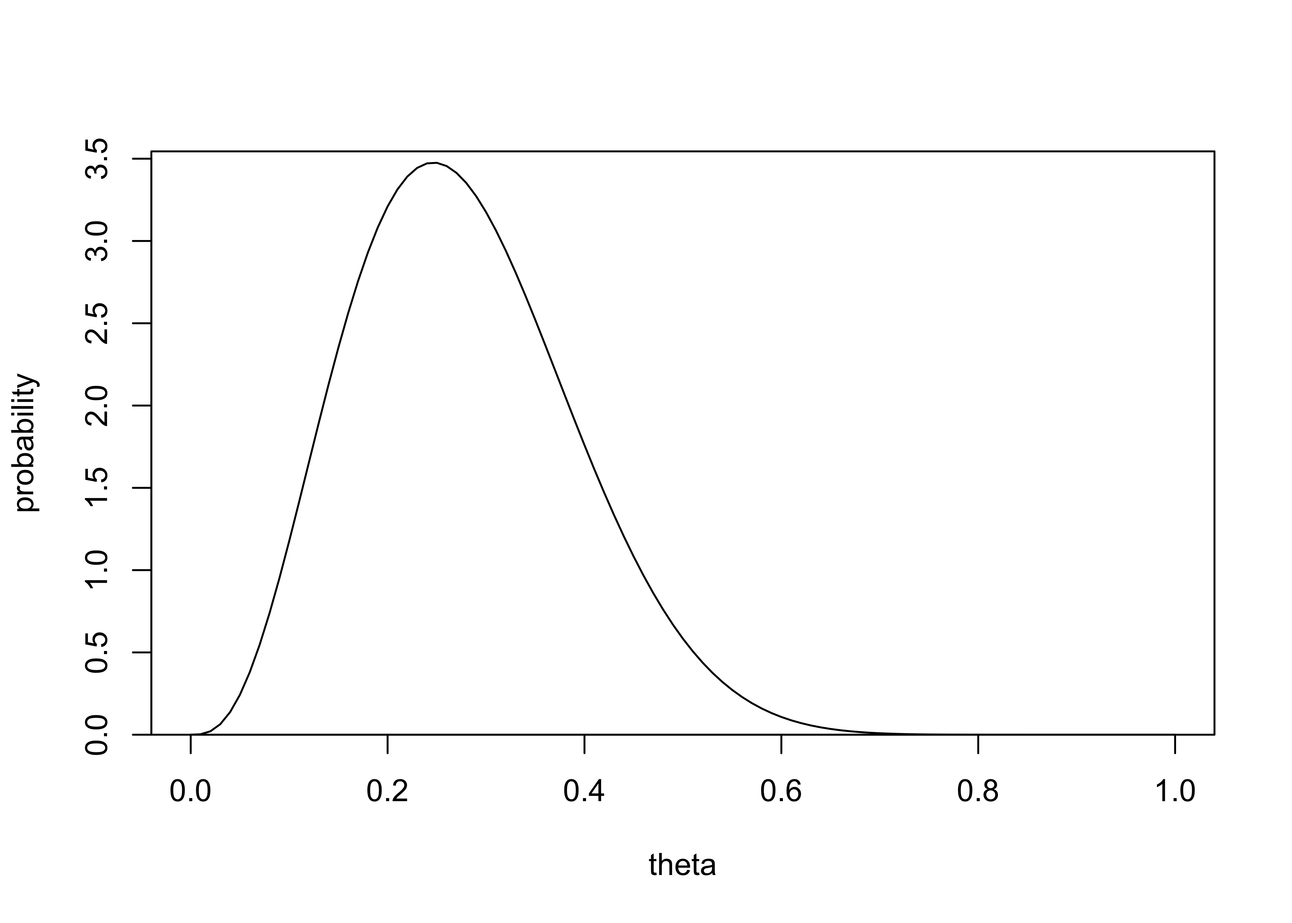
30.3 Question 2
Predictive distributions: consider two coins \(C_1\) and \(C_2\) with the following characteristics: \(\Pr(\text{heads} | C_1) = 0.6\) and \(\Pr(\text{heads} | C_2) = 0.4\). Choose one of the coins at random and spin it. Given that the first two spins are tails, what is the expectation of the number of additional spins until a heads?
Find the probability of each coin given the data and use those as “weights” for the expected number of spins to get heads.
\[ p(C_1|y) = \frac{p(C_1) p(y|C_1)}{p(y)} \\ p(C_1) = \frac{1}{2} \\ p(y|C_1) = (1-0.6)^2 = 0.4^2 = \frac{16}{100} \\ p(y) = \frac{1}{2} \frac{16}{100} + \frac{1}{2} \frac{36}{100} \\ p(C_1|y) = \frac{\frac{1}{2} \frac{16}{100}}{\frac{1}{2} \frac{16}{100} + \frac{1}{2} \frac{36}{100}} = \frac{8}{26} \] Same cacuation for \(p(C_2|y)\) resulting in \(p(C_2|y) = \frac{18}{26}\).
Expected number \(n\) of coin spins until get heads given the probability of getting heads \(\theta\):
\[ \text{E}(n|\theta) = 1 \theta + 2(1-\theta)\theta + 3(1 - \theta)^2 \theta + \dots = \frac{1}{\theta} \]
Thus
\[ \begin{aligned} \text{E}(n|y) &= p(C_1|y) \text{E}(n|C_1,y) + p(C_2|y) \text{E}(n|C_2,y) \\ &= \frac{8}{26} \frac{1}{0.6} + \frac{18}{26} \frac{1}{0.4} \\ &= 2.24 \end{aligned} \]
30.4 Question 3
Predictive distributions: let \(y\) be the number of 6’s in 1000 rolls of a fair die.
a) Sketch the approximate distribution of \(y\) based on the normal approximation.
mean: \(\text{E}(y) = \frac{1}{6} 1000 = \frac{500}{3}\)
std. dev: \(\text{sd}(y) = \sqrt{\frac{1}{6} \frac{5}{6} 1000}\)
mu <- 500 / 3
sigma <- sqrt(1000 * 5 / (6 * 6))
y <- seq(100, 250, 1)
likelihood <- dnorm(y, mu, sigma)
plot_dist(y, likelihood, xlab = "y", ylab = "likelihood")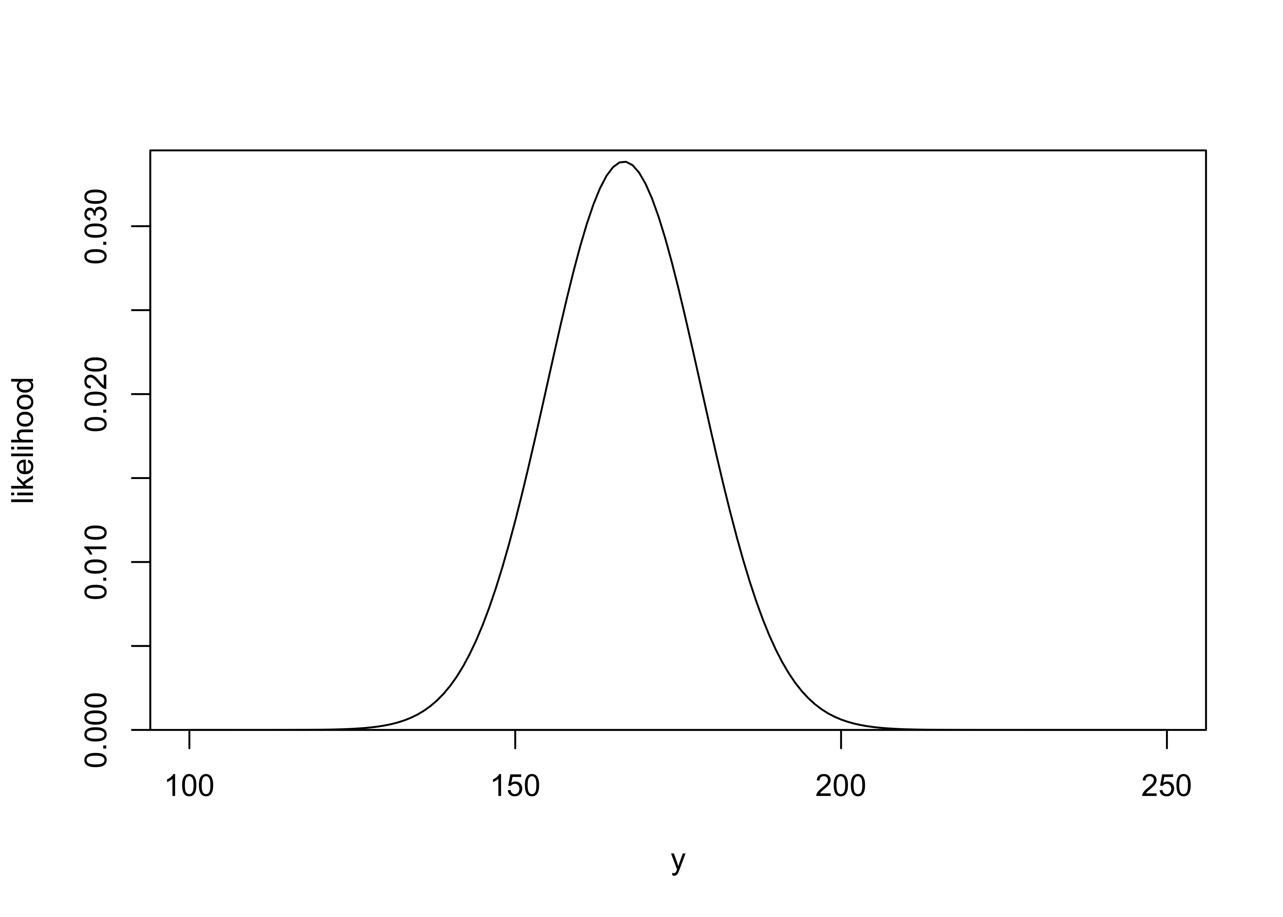
b) Using the normal distribution table, give approximate 5%, 25%, 50%, 75%, and 95% points for the distribution of \(y\).
| percentile | z | formula | value |
|---|---|---|---|
| 5% | -1.65 | \(\text{E}(y) - 1.65 \times \text{sd}(y)\) | 147.2 |
| 25% | -0.67 | \(\text{E}(y) - 1.65 \times \text{sd}(y)\) | 158.8 |
| 50% | 0 | \(\text{E}(y)\) | 166.7 |
| 75% | 0.67 | \(\text{E}(y) + 1.65 \times \text{sd}(y)\) | 174.6 |
| 95% | 1.65 | \(\text{E}(y) + 1.65 \times \text{sd}(y)\) | 186.1 |
p <- map_chr(c(5, 25, 50, 75, 95), ~ glue("{.x}%"))
q <- c(147.2, 158.8, 166.7, 174.6, 186.1)
pqs <- tibble(p = p, q = q)

d <- tibble(y = y, likelihood = likelihood)
ggplot(d, aes(x = y, y = likelihood)) +
  geom_line() +
  geom_vline(aes(xintercept = q, color = p), data = pqs, show.legend = FALSE) +
  geom_text(aes(x = q, label = p), data = pqs, y = 0.036, show.legend = FALSE) +
  scale_x_continuous(expand = expansion()) +
  scale_y_continuous(expand = expansion(mult = c(0, 0.1))) +
  theme_bw()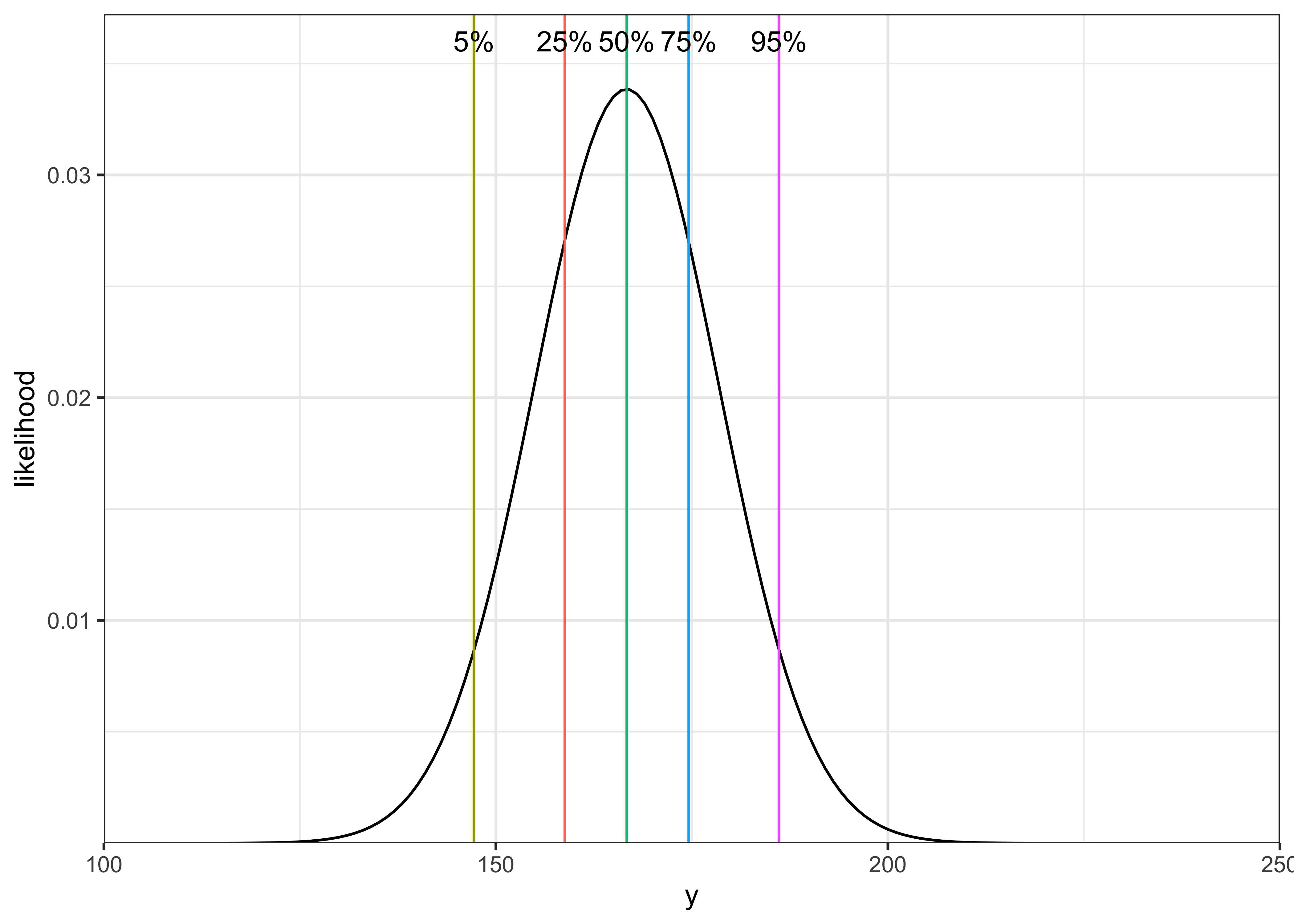
30.5 Question 4
Predictive distributions: let \(y\) be the number of 6’s in 1000 rolls of a die that may not be fair. Let \(\theta\) be the probability that the die lands on 6 with the following priors for different values of \(\theta\):
\[ \begin{aligned} \Pr(\theta = \frac{1}{12} &= 0.25) \\ \Pr(\theta = \frac{1}{6} &= 0.5) \\ \Pr(\theta = \frac{1}{4} &= 0.25) \\ \end{aligned} \]
a) Using the normal approximation for the conditional distributions \(p(y|\theta)\), sketch the prior predictive for \(y\).
prior predictive: \(p(\tilde{y}|M) = \int p(\tilde{y}|\theta, n, M) p(\theta|M)\)
for this exercise: \[ \begin{aligned} p(\tilde{y}|M) &= p(\tilde{y} | \theta=\frac{1}{12}, n=1000, M) p(\theta=\frac{1}{12}) + \dots \\ &= N(\frac{1}{12} 1000, \sqrt{1000 \frac{1}{12} (1 - \frac{1}{12})}) \times \frac{1}{4} + \dots \\ \end{aligned} \]
six_likelihood <- function(y, theta, n = 1000, prior) {
  mu <- n * theta
  sigma <- sqrt(n * theta * (1 - theta))
  dnorm(y, mu, sigma) * prior
}

y <- seq(30, 310)
separate_likelihoods <- map2(
  c(1 / 12, 1 / 6, 1 / 4),
  c(0.25, 0.5, 0.25),
  ~ six_likelihood(y, .x, n = 1000, prior = .y)
)

combined_likelihood <- accumulate(separate_likelihoods, ~ .x + .y)[[3]]

plot_dist(y, combined_likelihood, "y", "likelihood")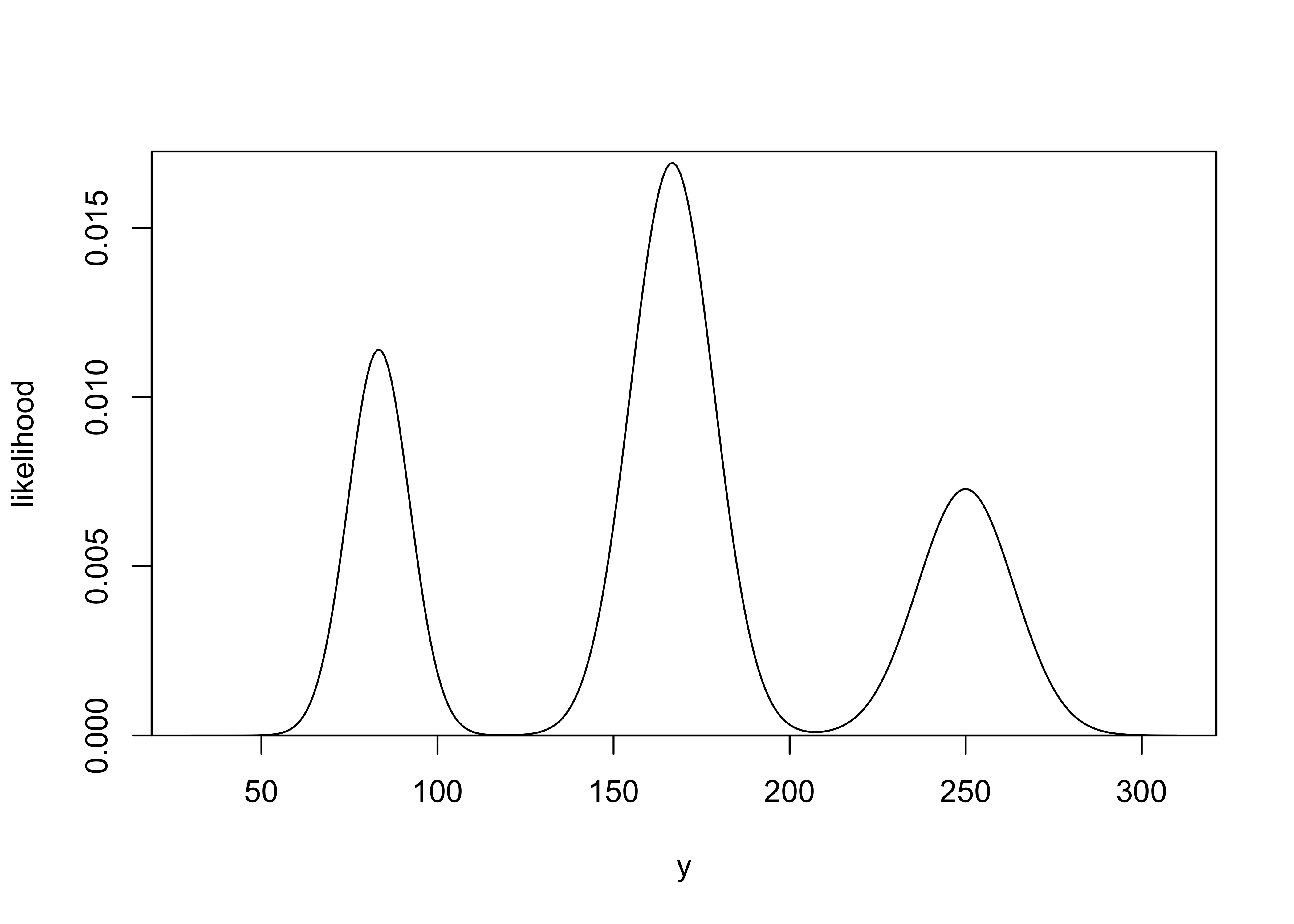
sessionInfo()#> R version 4.1.2 (2021-11-01)
#> Platform: x86_64-apple-darwin17.0 (64-bit)
#> Running under: macOS Big Sur 10.16
#>
#> Matrix products: default
#> BLAS: /Library/Frameworks/R.framework/Versions/4.1/Resources/lib/libRblas.0.dylib
#> LAPACK: /Library/Frameworks/R.framework/Versions/4.1/Resources/lib/libRlapack.dylib
#>
#> locale:
#> [1] en_US.UTF-8/en_US.UTF-8/en_US.UTF-8/C/en_US.UTF-8/en_US.UTF-8
#>
#> attached base packages:
#> [1] stats graphics grDevices datasets utils methods base
#>
#> other attached packages:
#> [1] forcats_0.5.1 stringr_1.4.0 dplyr_1.0.7 purrr_0.3.4
#> [5] readr_2.0.1 tidyr_1.1.3 tibble_3.1.3 ggplot2_3.3.5
#> [9] tidyverse_1.3.1 glue_1.4.2
#>
#> loaded via a namespace (and not attached):
#> [1] Rcpp_1.0.7 lubridate_1.7.10 here_1.0.1 clisymbols_1.2.0
#> [5] assertthat_0.2.1 rprojroot_2.0.2 digest_0.6.27 utf8_1.2.2
#> [9] R6_2.5.0 cellranger_1.1.0 backports_1.2.1 reprex_2.0.1
#> [13] evaluate_0.14 httr_1.4.2 highr_0.9 pillar_1.6.2
#> [17] rlang_0.4.11 readxl_1.3.1 rstudioapi_0.13 jquerylib_0.1.4
#> [21] rmarkdown_2.10 labeling_0.4.2 munsell_0.5.0 broom_0.7.9
#> [25] compiler_4.1.2 modelr_0.1.8 xfun_0.25 pkgconfig_2.0.3
#> [29] htmltools_0.5.1.1 tidyselect_1.1.1 bookdown_0.24 fansi_0.5.0
#> [33] crayon_1.4.1 tzdb_0.1.2 dbplyr_2.1.1 withr_2.4.2
#> [37] grid_4.1.2 jsonlite_1.7.2 gtable_0.3.0 lifecycle_1.0.0
#> [41] DBI_1.1.1 magrittr_2.0.1 scales_1.1.1 cli_3.0.1
#> [45] stringi_1.7.3 farver_2.1.0 renv_0.14.0 fs_1.5.0
#> [49] xml2_1.3.2 bslib_0.2.5.1 ellipsis_0.3.2 generics_0.1.0
#> [53] vctrs_0.3.8 tools_4.1.2 hms_1.1.0 yaml_2.2.1
#> [57] colorspace_2.0-2 rvest_1.0.1 knitr_1.33 haven_2.4.3
#> [61] sass_0.4.0